
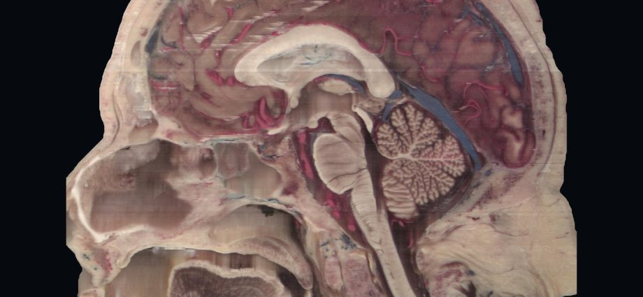
Anatomia da cabeça em 3D: rosto, crânio e cérebro de uma só pessoa
Anatomia da cabeça em 3D sem nada desenhado: tomografia e 1.477 cortes fotografados da mesma cabeça, doada à ciência, em um modelo para separar camadas, cortar, comparar exames e testar o que você sabe.
📅 Publicado em 4 de novembro de 2026
Navegue pelo Artigo
Do filme ao modelo, do modelo aos cortes, e de tudo isso ao passo a passo de como foi feito.
- 1. Por que ver a cabeça inteira
- 2. Assista: Atrás do Rosto
- 3. Explore a cabeça em 3D
- 4. As três incidências
- 5. O exame sobre a peça
- 6. De onde vem o material
- 7. Como foi feito, passo a passo
- 8. O que deu errado no caminho
- 9. Os números, sem filtro
- 10. O que é real e o que é reconstruído
- 11. Como usar isto no ensino
- 12. Perguntas frequentes
- 13. Considerações Finais
- 14. Referências
1. Por que ver a cabeça inteira
Para entender a anatomia da cabeça em 3D, todo médico aprende a montar um objeto mental a partir de fatias. A tomografia chega em cortes, o residente percorre a pilha e, depois de alguns anos, passa a enxergar volume onde antes via tons de cinza. Ninguém ensina esse salto de forma direta. Ele acontece, ou demora.
Este material foi feito para encurtar o caminho. O filme começa em um rosto, tira a pele, mostra o crânio e entra no cérebro por planos que giram. Abaixo dele há um modelo que você mesmo pode desmontar: tirar a pele, afastar o crânio, cortar em qualquer plano e, no fim, fazer uma prova com a peça real. Tudo vem de uma única pessoa, um homem de 72 anos que doou o corpo à ciência.
2. Assista: Atrás do Rosto
São 93 segundos, em duas vozes. Perto do fim, uma régua dourada mede, nesta cabeça, a distância da pele da testa até o corpo caloso.
3. Explore a cabeça em 3D
Clique para abrir (são 5,3 MB, e o carregamento pode levar alguns segundos). No computador, mais 7,4 MB chegam em segundo plano e deixam tudo mais nítido. À esquerda fica a cabeça em 3D; à direita, os cortes axial, coronal e sagital, mais um quarto painel com o mesmo plano no outro exame.
Comece pelas camadas: pele e tecidos moles, crânio, e encéfalo com meninges se afastam na mesma escala e giram juntos. Depois clique em qualquer ponto de qualquer corte. Os outros painéis e o 3D acompanham, como no cursor de uma estação de laudo, só que aqui a imagem ao lado da tomografia é a peça real. Se o clique cair perto de uma das 53 estruturas marcadas, ela é explicada embaixo, com a distância até a pele da testa e os vizinhos anatômicos em botões. Setas ligam cada legenda à estrutura, e linhas tracejadas ligam a estrutura escolhida aos vizinhos no mesmo plano. Dá para ir de vizinho em vizinho.
E quando achar que já sabe, abra o Autoteste. As legendas somem. O modelo marca uma estrutura e pede o nome, ou dá o nome e pede o clique no lugar certo. São dez perguntas, com a explicação anatômica a cada resposta e, no fim, a lista do que revisar. Dá para treinar a cabeça inteira, só o encéfalo, só os vasos ou só a face.
Cinco coisas para experimentar
4. As três incidências
Os cortes abaixo são fotos da própria peça, em resolução cheia. No axial aparecem os olhos, a ponte e o cerebelo no mesmo plano. No coronal, os ventrículos laterais e os lobos temporais. No sagital, o corpo caloso, o tronco, a medula e a árvore do cerebelo.

Como ler as três incidências
Axial separa o que está em cima do que está embaixo. Coronal separa frente e trás. Sagital separa direita e esquerda. Só o axial foi fotografado; coronal e sagital são reformatações da mesma pilha, como as que o PACS faz.
5. O exame sobre a peça
À esquerda, a tomografia. À direita, a peça, no mesmo plano. O osso da TC continua sobre o crânio do corte real, e essa continuidade foi o teste do alinhamento. O exame traduz em tons de cinza a densidade de um tecido que tem cor, textura e vasos.

6. De onde vem o material
A base é a coleção Additional Head Images, do Visible Human Project da National Library of Medicine dos EUA. É um projeto posterior ao homem e à mulher mais conhecidos da NLM, descrito por Ratiu e colaboradores como Visible Human 2.0 [1,2].
A cabeça e o pescoço de um doador de 72 anos foram fixados em formol, e os sistemas arterial e venoso foram injetados com araldite colorida. Antes do congelamento, fizeram tomografia e ressonância com hardware de registro já inserido. Depois vieram os cortes, com pixel e espaçamento de 0,147 mm: 1.477 faces fotografadas, em imagens de 1056 × 1528 pixels [1,4].
Desde 2019 os dados são públicos, sem licença, com crédito obrigatório à NLM [3,5].
A doação
Nada disso existiria sem uma decisão tomada em vida. Por isso o filme diz que foi uma doação, informa a idade do doador e não usa nenhum outro dado pessoal.
7. Como foi feito, passo a passo
Trabalhei com o Claude Code como executor, sob a Metodologia AIMED: eu defini o objetivo, revisei cada etapa e aprovei imagem, roteiro e áudio. Todo o código ficou guardado e pode ser refeito. A ordem real foi esta.
1. Baixar e conferir
Foram 2.245 arquivos da NLM, 291,6 MB: 1.477 cortes axiais em JPEG, 463 imagens de TC (pixel de 0,489 mm, corte de 0,5 mm), 229 de T2 e 76 de T1. O tamanho de cada arquivo foi conferido com o índice do servidor. Nenhuma divergência.
2. Montar o volume
Reduzi a pilha três vezes em cada eixo, por média. O resultado tem 492 × 509 × 352 voxels de 0,441 mm, o que cabe na memória de uma placa de vídeo integrada (Intel UHD 620, a deste notebook).
3. Separar a cabeça da placa
A peça foi fotografada sobre uma placa cinza. No espaço de cor Lab, o croma da placa é baixo, e o do tecido, mesmo a gordura pálida, é maior. Usei limiar de croma 9, abertura morfológica, maioria entre nove cortes vizinhos para eliminar falhas de um corte só, fechamento e preenchimento de buracos. Como a cabeça encosta nas bordas laterais da foto, precisei fechar o contorno artificialmente antes de preencher.
4. Trazer o rosto da tomografia
A foto dos cortes perdeu a ponta do nariz e as orelhas, porque a cabeça é maior que o quadro. A TC tem tudo isso. Alinhei a TC aos cortes por registro rígido: seis parâmetros (três translações, três rotações), otimizador de Powell, maximizando o coeficiente de Dice entre os contornos em grade de 1,76 mm, com três pontos de partida e as duas orientações possíveis. A versão espelhada venceu, 0,9628 contra 0,9567. Rotações abaixo de 3,3° e translações de até 8,9 mm.
5. Retirar o hardware de registro
As hastes colocadas antes dos exames aparecem na TC. Tirei da superfície o que era fino e externo, com abertura morfológica corte a corte no topo e na base da cabeça, onde o corte é sólido. No nariz, nos lábios e nas orelhas não toquei.
6. Separar as camadas
O crânio é o osso da TC, por limiar. O conteúdo intracraniano veio de uma ideia simples: é o espaço fechado pelo osso. Calculei a distância de cada voxel até o osso, guardei só o que fica a mais de 8,8 mm (isso fecha forames e canal medular), tomei a região que contém um ponto dentro do cérebro e a fiz crescer de volta até o osso. O contorno acompanhou a face interna do crânio nos três planos. São 1.660 mL, número que inclui meninges, líquor, vasos e o início da medula. O restante da cabeça é a camada de pele e tecidos moles.
7. Renderizar o filme
Escrevi um raymarching em ModernGL: para cada pixel, um raio caminha pelo volume em passos de cerca de 0,5 mm até encontrar a pele, o osso ou o plano de corte. Na superfície, a luz vem do gradiente da máscara. Na face do corte, a cor é a da foto. Foram 2.249 quadros a 24 por segundo, em 810 × 1440, ampliados para 1080 × 1920. Levou cerca de dez minutos.
8. Voz, legenda e trilha
As vozes saíram do Google AI Studio (Gemini TTS, Kore e Zubenelgenubi), uma geração por idioma: 71,96 s em português, 82,88 s em inglês. Como o inglês é mais longo, cada fala ganhou o tempo do idioma mais lento; assim a imagem é idêntica nos dois filmes e foi renderizada uma vez só. O faster-whisper deu o tempo real de cada palavra, para as legendas. A trilha é “With These Hands”, de Scott Buckley, com ducking sob as vozes e cerca de −16 LUFS.
9. Levar o modelo para o navegador
O volume foi reduzido para 0,88 mm e empacotado em 246 cortes por atlas: um para a cor, um para a TC, um para as máscaras. São dois arquivos que somam 5,3 MB. No computador, a cor é trocada em segundo plano por uma versão de 0,59 mm, em mais 7,4 MB; no celular fica a versão leve, para não estourar a memória. No seu navegador, tudo vira textura 3D em WebGL2 e o mesmo raymarching roda ali, em tempo real. Os painéis 2D são reformatados do mesmo volume a cada clique.
10. Marcar as estruturas
Gerei planos com régua e marquei à mão 53 pontos, olhando a imagem real, cada um com texto curto e vizinhos anatômicos. Depois conferi todos: recortes nos três planos, auditoria por cor e densidade e séries de cortes nas regiões difíceis. Achei seis erros meus. Uma cartilagem da tuba auditiva tinha virado dente; um côndilo occipital tinha virado atlas, até eu contar as vértebras a partir do dente do áxis.
11. Ligar tudo
Cada legenda fica na margem, com uma seta até a estrutura, e só aparece se a face do corte estiver voltada para quem olha. Cada corte mostra a estrutura escolhida, os vizinhos e as mais próximas; as outras viram pontos clicáveis. Os painéis leem o mesmo volume do 3D, e por isso um clique move tudo junto.
12. Transformar em prova
O autoteste usa os mesmos 53 pontos. Sorteia dez, alterna as duas formas de pergunta e separa o que é compacto do que é extenso: ninguém deveria errar por clicar em outra parte de um lobo, então lobos e músculos só entram na pergunta de nome. Nada do que você responde sai do seu navegador.
8. O que deu errado no caminho
Quase tudo o que você vê passou por uma versão ruim antes.
A geada da placa criava uma coroa falsa no topo da cabeça. Minha primeira correção deixou o crânio em forma de cone. A solução real veio só depois, quando a TC passou a definir o contorno externo.
Num teste, a tomografia cobriu o filme inteiro até o fim: uma cortina que deveria voltar seguia para o lado errado, por um sinal trocado. Só vi na folha de contato com dezesseis quadros, e por isso não confio em um quadro só.
A pele do modelo interativo saiu manchada, em mosaico. Eu tinha reduzido a máscara a 16 níveis para economizar bytes e calculava a luz sobre ela. Passei a 64 níveis e a usar o campo contínuo.
As legendas sobrepostas sumiam: desenhar texto transparente na biblioteca de imagens apaga o que está embaixo, em vez de não fazer nada.
E as hastes. Chamei-as de pinos até ler o artigo original, que explica que são o hardware de registro [1]. A leitura do paper veio tarde demais para o roteiro, a tempo do artigo.
O modelo travava a aba do Chrome ao abrir. O compilador de shaders do Windows tentava desenrolar um laço de 1.300 passos; bastou trocar a forma de ler a textura para abrir em cerca de 8 segundos neste notebook.
Ao girar a cabeça, as legendas do corte continuavam flutuando por cima da pele, apontando para o nada. E as fotos pareciam borradas, até eu criar a camada de 0,59 mm. Os dois defeitos apareceram na minha revisão do rascunho, usando o modelo como um aluno usaria.
9. Os números, sem filtro
| Medida | Valor | Como foi obtida |
|---|---|---|
| Cortes | 1.477 | Documentação da NLM |
| Pixel e espaçamento | 0,147 mm | Documentação da NLM |
| Pele até o osso, na testa | 5,7 mm | TC alinhada, linha média |
| Pele da testa até o joelho do corpo caloso | cerca de 6,5 cm (64,4 a 64,8 mm) | TC e corte real, linha média; estrutura localizada por cor |
| Comprimento da cabeça, nesse nível | 204 mm | Contorno da TC |
| Espaço intracraniano segmentado | 1.660 mL | TC; inclui meninges, líquor, vasos e início da medula |
| Sobreposição TC × cortes | Dice 0,96 | Registro rígido, grade de 1,76 mm |
| Estruturas marcadas no modelo | 53 | Marcação manual, com conferência em três planos |
São medidas de um único doador adulto, em peça fixada. Dão escala a este material e não valem como referência populacional, muito menos pediátrica. As distâncias mostradas no modelo são linhas retas entre pontos marcados à mão, com a precisão de um clique.
10. O que é real e o que é reconstruído
⚠ O que é real e o que é reconstruído
Reais: as fotos dos cortes, as imagens da tomografia e a forma do rosto e do crânio.
Reconstruídos: os planos coronal, sagital e oblíquo, calculados a partir dos cortes axiais, e o volume 3D, reduzido a 0,441 mm no filme e a 0,59 mm ou 0,88 mm no modelo. As figuras do artigo têm a resolução original.
Escolhida no render: a cor da pele e do osso, que vêm da TC e não têm cor própria.
Tratados: a cor do tecido é a de uma peça fixada, e o vermelho e o azul dos vasos vêm da resina; quatro cortes da coleção são médias calculadas pela própria NLM; o hardware de registro foi retirado da superfície, com vestígios na testa, no crânio e na mandíbula; a orelha esquerda está incompleta.
A camada de encéfalo inclui meninges, e sua forma é a da face interna do crânio, sem giros individualizados na superfície.
Não indiquei direita e esquerda nas imagens: o registro sugere que TC e fotos têm orientações espelhadas, e prefiro não afirmar lateralidade sem confirmação.
11. Como usar isto no ensino
Mostre primeiro a TC e peça ao residente que aponte uma estrutura; depois revele o corte real no mesmo plano. Com o modelo aberto, isso leva menos de um minuto, e a comparação ensina mais do que qualquer descrição verbal minha.
A série já fez esse exercício com o coração, em Fontan em 3D, e a anatomia em 3D aparece também em O coração que eu posso abrir na tela. Os outros episódios estão na coleção Cinematic Education.
12. Perguntas frequentes
O que é o Visible Human Project?
É um projeto da National Library of Medicine dos EUA que disponibiliza imagens anatômicas de corpos doados: fotos de cortes, tomografia e ressonância. Desde 2019 o acesso não exige licença, com crédito obrigatório à NLM.
Este modelo 3D da cabeça é de uma pessoa real?
Sim. Rosto e crânio vêm da tomografia, e as faces de corte vêm de fotos da peça de um doador de 72 anos. A cor da pele e do osso foi escolhida no render.
Qual a diferença entre corte axial, coronal e sagital?
O axial divide o corpo em cima e embaixo, o coronal em frente e trás, e o sagital em direita e esquerda. No modelo, um clique em qualquer um deles move os outros dois.
O modelo funciona no celular?
Funciona em navegadores com WebGL2 e carrega 5,3 MB depois do clique, em uma versão mais leve que a do computador. Em telas pequenas, os painéis ficam abaixo do 3D.
Como estudar neuroanatomia com este modelo?
Siga os nove passos guiados, escolha uma estrutura e percorra os vizinhos pelos botões. Depois feche as legendas e faça o autoteste. Repita na semana seguinte: a lista de revisão mostra onde insistir.
Posso usar em aula?
Pode, abrindo esta página e citando a fonte. O material é educativo, de um único adulto, e não serve para diagnóstico nem para planejamento cirúrgico.
Quer aprender a construir materiais assim?
A Metodologia AIMED organiza como pedir, conferir e documentar o trabalho com IA, do roteiro ao dado.
13. Considerações Finais
O que torna este material difícil de repetir é a soma: um conjunto pouco usado, exames alinhados, camadas segmentadas, motor próprio, 53 estruturas conferidas, relações clicáveis e uma prova sobre a peça real. Cada parte existe em algum lugar. Juntas, em um navegador, eu ainda não tinha visto. Quando for estudar cérebro, volte aqui.
💡 Connecting the Dots: o exame e o corpo são a mesma coisa vista de dois jeitos. Da próxima vez que abrir uma tomografia de crânio com um residente, tente abrir este modelo ao lado. E lembre que só temos essa ponte porque um homem de 72 anos decidiu doar.
Referências
- Ratiu P, Hillen B, Glaser J, Jenkins DP. Visible Human 2.0: the next generation. Stud Health Technol Inform. 2003;94:275-81. PMID: 15455907.
- Spitzer V, Ackerman MJ, Scherzinger AL, Whitlock D. The Visible Human Male: a technical report. J Am Med Inform Assoc. 1996;3(2):118-30. DOI: 10.1136/jamia.1996.96236280.
- U.S. National Library of Medicine. The Visible Human Project: Getting the Data. Disponível em: nlm.nih.gov/research/visible/getting_data.html.
- U.S. National Library of Medicine. Additional Head Images (README). Disponível em: data.lhncbc.nlm.nih.gov.
- U.S. National Library of Medicine. Terms and Conditions. Disponível em: nlm.nih.gov/databases/download/terms_and_conditions.html.
Courtesy of the U.S. National Library of Medicine. A NLM não endossa este trabalho. Música do filme: “With These Hands” by Scott Buckley, released under CC-BY 4.0. www.scottbuckley.com.au.
Head anatomy in 3D: the face, skull and brain of one person
Head anatomy in 3D with nothing drawn: CT and 1,477 photographed slices of the same head, donated to science, in a model to separate layers, cut, compare exams and test what you know.
📅 Published November 4, 2026
Table of Contents
From the film to the model, from the model to the slices, and from all that to how it was made, step by step.
- 1. Why see the whole head
- 2. Watch: Behind the Face
- 3. Explore the head in 3D
- 4. The three planes
- 5. The scan over the specimen
- 6. Where the material comes from
- 7. How it was made, step by step
- 8. What went wrong along the way
- 9. The numbers, unfiltered
- 10. What is real and what is reconstructed
- 11. How to use this in teaching
- 12. Frequently asked questions
- 13. Final Considerations
- 14. References
1. Why see the whole head
To grasp head anatomy in 3D, every physician learns to build a mental object from slices. CT arrives as sections, the resident scrolls through the stack and, after a few years, begins to see volume where there were only shades of gray. Nobody teaches that leap directly. It happens, or it takes a long time.
This material was made to shorten the path. The film starts with a face, removes the skin, shows the skull and enters the brain through rotating planes. Below it is a model you can take apart yourself: remove the skin, move the skull aside, cut in any plane and, at the end, sit a test on the real specimen. It all comes from one person, a 72-year-old man who donated his body to science.
2. Watch: Behind the Face
It runs 93 seconds, in two voices. Near the end, a gold ruler measures, in this head, the distance from the forehead skin to the corpus callosum.
3. Explore the head in 3D
Click to open it (5.3 MB, and loading can take a few seconds). On a computer, another 7.4 MB arrive in the background and sharpen everything. The 3D head is on the left; on the right are the axial, coronal and sagittal slices, plus a fourth panel with the same plane on the other exam.
Start with the layers: skin and soft tissue, skull, and brain with meninges move apart at the same scale and rotate together. Then click any point on any slice. The other panels and the 3D view follow, like the cursor on a reading workstation, except that the image beside the CT is the real specimen. If the click lands near one of the 53 marked structures, it is explained below, with its distance from the forehead skin and its anatomical neighbors as buttons. Arrows link each label to its structure, and dashed lines link the chosen structure to its neighbors in the same plane. You can walk from neighbor to neighbor.
And when you think you know it, open the Self-test. The labels disappear. The model marks a structure and asks for its name, or gives the name and asks you to click the right place. There are ten questions, with an anatomical explanation after each answer and, at the end, a list of what to review. You can train the whole head, only the brain, only the vessels or only the face.
Five things to try
4. The three planes
The sections below are full-resolution photographs of the specimen itself. The axial plane shows the eyes, pons and cerebellum together. The coronal plane shows the lateral ventricles and temporal lobes. The sagittal plane shows the corpus callosum, brainstem, spinal cord and the tree of the cerebellum.

How to read the three planes
Axial separates up from down. Coronal separates front from back. Sagittal separates right from left. Only the axial plane was photographed; coronal and sagittal are reformats of the same stack, as a PACS produces.
5. The scan over the specimen
CT on the left. The specimen on the right, in the same plane. The CT bone continues over the skull of the real slice, and that continuity was the test of the alignment. The scan translates into shades of gray the density of a tissue that has color, texture and vessels.

6. Where the material comes from
The source is the Additional Head Images collection of the Visible Human Project at the U.S. National Library of Medicine. It came after the NLM’s better-known male and female, and Ratiu and colleagues describe it as Visible Human 2.0 [1,2].
The head and neck of a 72-year-old donor were fixed in formalin, and the arterial and venous systems were injected with colored araldite. Before freezing, CT and MRI were acquired with registration hardware already inserted. Then came the sections, with 0.147 mm pixels and spacing: 1,477 photographed faces, in images of 1056 × 1528 pixels [1,4].
Since 2019 the data have been public, with no license, and credit to the NLM is required [3,5].
The donation
None of this would exist without a decision made in life. That is why the film says it was a donation, gives the donor’s age and uses no other personal data.
7. How it was made, step by step
I worked with Claude Code as the executor, under the AIMED Methodology: I set the goal, reviewed each stage and approved image, script and audio. All the code was kept and can be rerun. This was the actual order.
1. Download and check
2,245 files from the NLM, 291.6 MB: 1,477 axial sections in JPEG, 463 CT images (0.489 mm pixels, 0.5 mm slices), 229 T2 and 76 T1. Each file size was checked against the server index. No discrepancies.
2. Build the volume
I reduced the stack threefold on each axis, by averaging. The result has 492 × 509 × 352 voxels of 0.441 mm, which fits the memory of an integrated graphics chip (Intel UHD 620, the one in this laptop).
3. Separate the head from the plate
The specimen was photographed on a gray plate. In Lab color space, the plate has low chroma, and tissue, even pale fat, has more. I used a chroma threshold of 9, morphological opening, a majority vote across nine neighboring sections to remove single-section failures, closing and hole filling. Because the head touches the side edges of the photo, I had to close the outline artificially before filling.
4. Bring the face from CT
The section photographs lost the tip of the nose and the ears, because the head is larger than the frame. CT has all of that. I aligned CT to the sections by rigid registration: six parameters (three translations, three rotations), Powell’s optimizer, maximizing the Dice coefficient between outlines on a 1.76 mm grid, from three starting points and both possible orientations. The mirrored version won, 0.9628 against 0.9567. Rotations stayed under 3.3° and translations up to 8.9 mm.
5. Remove the registration hardware
The rods placed before imaging show on CT. I removed what was thin and external, with slice-by-slice morphological opening at the top and base of the head, where the section is solid. I left the nose, lips and ears alone.
6. Separate the layers
The skull is CT bone, by threshold. The intracranial content came from a simple idea: it is the space enclosed by bone. I computed each voxel’s distance to bone, kept only what lay more than 8.8 mm away (this closes foramina and the spinal canal), took the region containing a point inside the brain and grew it back to the bone. The outline followed the inner surface of the skull in all three planes. It measures 1,660 mL, a figure that includes meninges, CSF, vessels and the start of the spinal cord. The rest of the head is the skin and soft tissue layer.
7. Render the film
I wrote a raymarcher in ModernGL: for each pixel, a ray walks through the volume in steps of about 0.5 mm until it meets skin, bone or the cutting plane. On surfaces, light comes from the mask gradient. On the cut face, the color is the photograph’s. That made 2,249 frames at 24 per second, at 810 × 1440, upscaled to 1080 × 1920. It took about ten minutes.
8. Voice, captions and music
The voices came from Google AI Studio (Gemini TTS, Kore and Zubenelgenubi), one generation per language: 71.96 s in Portuguese, 82.88 s in English. Because English runs longer, each line got the time of the slower language; the picture is identical in both films and was rendered only once. faster-whisper gave the real time of each word for the captions. The music is “With These Hands” by Scott Buckley, ducked under the voices at about −16 LUFS.
9. Take the model to the browser
The volume was reduced to 0.88 mm and packed as 246 sections per atlas: one for color, one for CT, one for masks. Two files add up to 5.3 MB. On a computer, color is replaced in the background by a 0.59 mm version, in another 7.4 MB; phones keep the light version to spare memory. In your browser it all becomes 3D textures in WebGL2 and the same raymarcher runs there, in real time. The 2D panels are reformatted from the same volume at each click.
10. Mark the structures
I generated planes with rulers and marked 53 points by hand, looking at the real image, each with a short text and anatomical neighbors. Then I checked them all: crops in three planes, an audit by color and density, and slice series in the hard regions. I found six of my own errors. Auditory tube cartilage had become a tooth; an occipital condyle had become the atlas, until I counted vertebrae from the dens.
11. Link everything
Each label sits in the margin, with an arrow to its structure, and appears only if the cut face is turned toward the viewer. Each slice shows the chosen structure, its neighbors and the closest ones; the others become clickable dots. The panels read the same volume as the 3D view, which is why one click moves everything.
12. Turn it into a test
The self-test uses the same 53 points. It draws ten, alternates the two question types and separates compact from extensive structures: nobody should lose a point for clicking another part of a lobe, so lobes and muscles appear only in the naming question. Nothing you answer leaves your browser.
8. What went wrong along the way
Almost everything you see went through a bad version first.
Frost on the plate created a false crown on top of the head. My first fix left the skull shaped like a cone. The real solution came only later, when CT began to define the outer outline.
In one test, CT covered the whole film to the end: a curtain that should have returned kept going the wrong way, because of a flipped sign. I saw it only on a sixteen-frame contact sheet, which is why I do not trust a single frame.
The skin of the interactive model came out blotchy, like a mosaic. I had reduced the mask to 16 levels to save bytes and was computing light on it. I moved to 64 levels and to the continuous field.
Overlaid captions kept vanishing: drawing transparent text in the image library erases what lies beneath, where it should do nothing.
And the rods. I called them pins until I read the original paper, which explains they are registration hardware [1]. That reading came too late for the script, in time for this article.
The model froze the Chrome tab on opening. The Windows shader compiler was trying to unroll a 1,300-step loop; changing how the texture is read brought opening down to about 8 seconds on this laptop.
When the head rotated, the slice labels kept floating over the skin, pointing at nothing. And the photographs looked blurry, until I built the 0.59 mm layer. Both flaws surfaced in my own draft review, using the model the way a student would.
9. The numbers, unfiltered
| Measure | Value | How it was obtained |
|---|---|---|
| Sections | 1,477 | NLM documentation |
| Pixel and spacing | 0.147 mm | NLM documentation |
| Skin to bone, at the forehead | 5.7 mm | Aligned CT, midline |
| Forehead skin to genu of the corpus callosum | about 6.5 cm (64.4 to 64.8 mm) | CT and real section, midline; structure located by color |
| Head length at that level | 204 mm | CT outline |
| Segmented intracranial space | 1,660 mL | CT; includes meninges, CSF, vessels and start of the spinal cord |
| CT × sections overlap | Dice 0.96 | Rigid registration, 1.76 mm grid |
| Structures marked in the model | 53 | Manual marking, checked in three planes |
These measures come from a single adult donor, in a fixed specimen. They give scale to this material and do not serve as a population reference, much less a pediatric one. The distances shown in the model are straight lines between points marked by hand, as precise as a click.
10. What is real and what is reconstructed
⚠ What is real and what is reconstructed
Real: the section photographs, the CT images and the shape of the face and skull.
Reconstructed: the coronal, sagittal and oblique planes, computed from the axial sections, and the 3D volume, reduced to 0.441 mm in the film and 0.59 mm or 0.88 mm in the model. The article figures keep the original resolution.
Chosen in the render: the color of skin and bone, which come from CT and have no color of their own.
Treated: tissue color is that of a fixed specimen, and the red and blue of the vessels come from resin; four sections in the collection are averages computed by the NLM itself; the registration hardware was removed from the surface, leaving traces on the forehead, skull and mandible; the left ear is incomplete.
The brain layer includes meninges, and its shape is that of the inner skull, with no individual gyri on the surface.
I did not mark right and left on the images: the registration suggests CT and photographs have mirrored orientations, and I prefer not to state laterality without confirmation.
11. How to use this in teaching
Show the CT first and ask the resident to point to a structure; then reveal the real slice in the same plane. With the model open, this takes less than a minute, and the comparison teaches more than any verbal description of mine.
The series has done this exercise with the heart, in Fontan in 3D, and 3D anatomy also appears in A heart I can open on screen. The other episodes are in the Cinematic Education collection.
12. Frequently asked questions
What is the Visible Human Project?
It is a U.S. National Library of Medicine project that provides anatomical images of donated bodies: section photographs, CT and MRI. Since 2019 access requires no license, with credit to the NLM.
Is this 3D head model from a real person?
Yes. The face and skull come from CT, and the cut faces come from photographs of a 72-year-old donor’s specimen. Skin and bone color were chosen in the render.
What is the difference between axial, coronal and sagittal planes?
Axial divides the body into upper and lower, coronal into front and back, and sagittal into right and left. In the model, a click on any of them moves the other two.
Does the model work on a phone?
It works in browsers with WebGL2 and loads 5.3 MB after the click, in a lighter version than on a computer. On small screens, the panels sit below the 3D view.
How do I study neuroanatomy with this model?
Follow the nine guided steps, choose a structure and walk through its neighbors with the buttons. Then turn the labels off and take the self-test. Repeat it the next week: the review list shows where to insist.
Can I use it in class?
Yes, by opening this page and citing the source. It is educational material from one adult and is not for diagnosis or surgical planning.
Want to learn how to build material like this?
The AIMED Methodology organizes how to ask, check and document work with AI, from script to data.
13. Final Considerations
What makes this material hard to repeat is the sum: a little-used dataset, aligned exams, segmented layers, a custom engine, 53 checked structures, clickable relations and a test on the real specimen. Each part exists somewhere. Together, in a browser, I had not seen them yet. When you next study the brain, come back here.
💡 Connecting the Dots: the scan and the body are the same thing seen in two ways. Next time you open a head CT with a resident, try opening this model beside it. And remember that we only have this bridge because a 72-year-old man decided to donate.
References
- Ratiu P, Hillen B, Glaser J, Jenkins DP. Visible Human 2.0: the next generation. Stud Health Technol Inform. 2003;94:275-81. PMID: 15455907.
- Spitzer V, Ackerman MJ, Scherzinger AL, Whitlock D. The Visible Human Male: a technical report. J Am Med Inform Assoc. 1996;3(2):118-30. DOI: 10.1136/jamia.1996.96236280.
- U.S. National Library of Medicine. The Visible Human Project: Getting the Data. Available at: nlm.nih.gov/research/visible/getting_data.html.
- U.S. National Library of Medicine. Additional Head Images (README). Available at: data.lhncbc.nlm.nih.gov.
- U.S. National Library of Medicine. Terms and Conditions. Available at: nlm.nih.gov/databases/download/terms_and_conditions.html.
Courtesy of the U.S. National Library of Medicine. The NLM does not endorse this work. Film music: “With These Hands” by Scott Buckley, released under CC-BY 4.0. www.scottbuckley.com.au.
◆ Novidades
- Anatomia do olho em 3D: faça o teste do olhinho em um olho realNOVO
- Fontan em 3D: o caminho até o pulmão que não passa pelo coração
- Transposição das grandes artérias em 3D, com corações de verdade (e o erro que eu quase publiquei)